Simulating many particles: A spiral of spheres
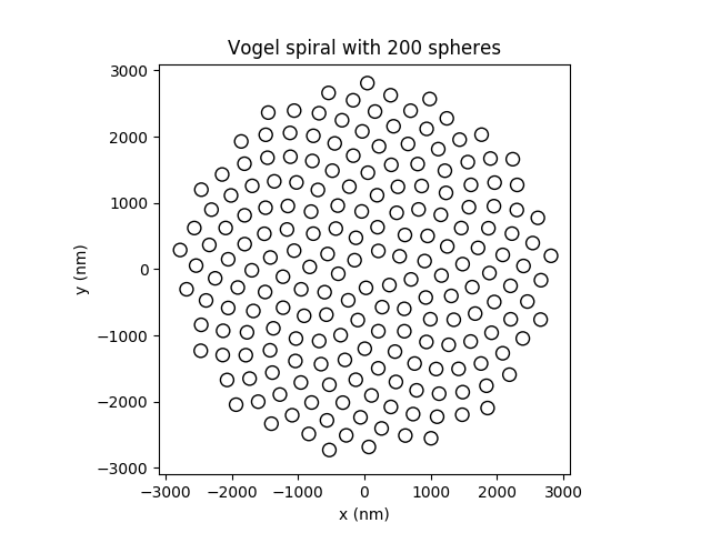
The configuration under study consists of a number of monodisperse dielectric spheres that are arranged in the shape of a spiral on a glass substrate. Please see the section on Solver settings for an overview on the different numerical approaches to solve the system of linear equations governing a Smuthi simulation.
The given configuration of particles is particularly well suited for the lookup table strategy, because all particle centers are on the same height (z-position) such that the interaction matrix can be calculated using a one-dimensional lookup table, see section 3.10.1.2 of Amos Egel’s PhD thesis.
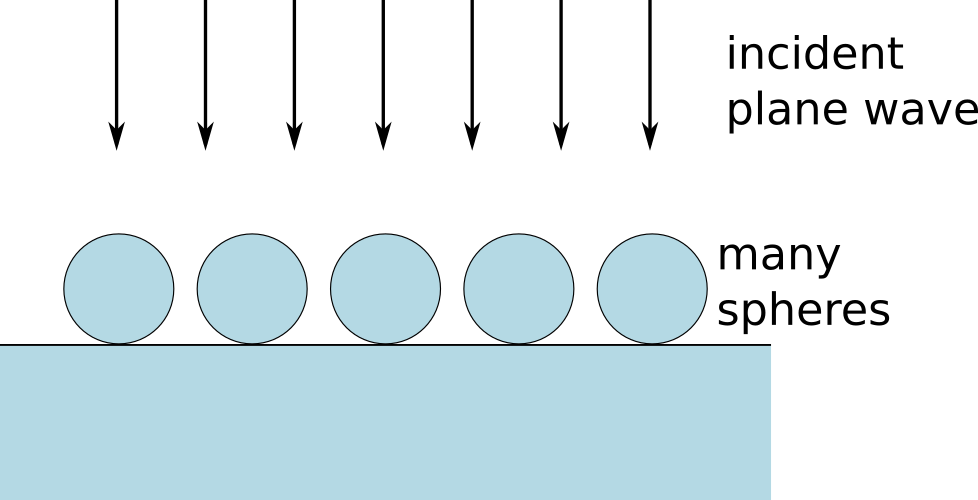
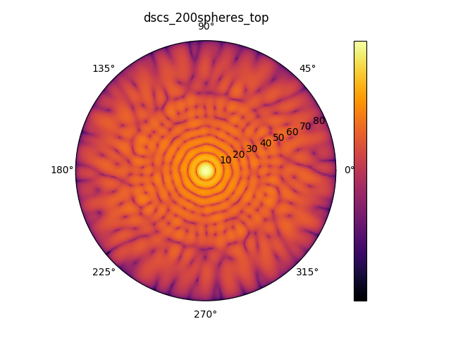
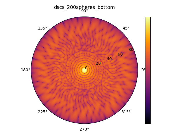
The spheres are illuminated by a plane wave from top under normal incidence. The resulting differential far field distribution of the scattered field for a spiral of 200 spheres is depicted below, both in the top hemisphere (reflection, left) and in the bottom hemisphere (transmission, right).
Let us discuss the runtime required by the solution of the scattering problem. In the
tutorial script,
we loop over the particle number and solve the scattering problem either with …
- direct solution (LU factorization) and explicit calculation of the coupling matrix
- iterative solution and linear interpolation of 1D lookup table on the CPU
- iterative solution and linear interpolation of 1D lookup table on the GPU.
In either case we measure the time that the algorithm needs to set up and and solve the system of linear equations.
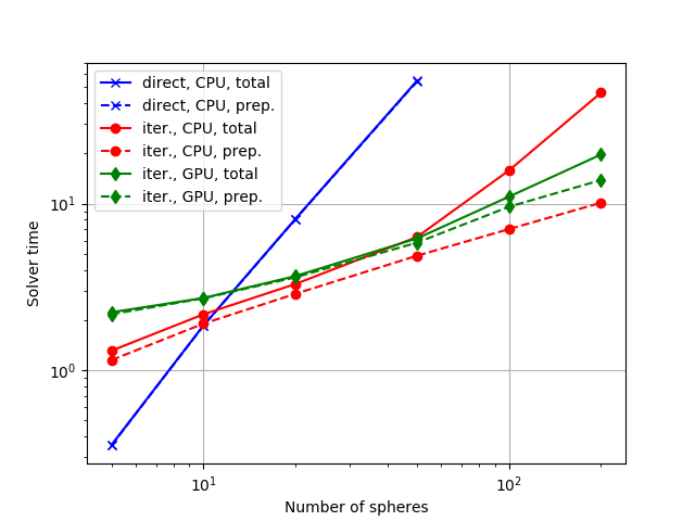
As the above figure illustrates, the direct solver is fastest for very small particle numbers (below ~10). Linear interpolation from a lookup table in conjunction with the iterative solver runs much faster for larger particle numbers. We can also see that the benefit from parallelization on the GPU starts to overcompensate the time losses due to overhead from memory transfer starting from ~100 particles.
Note
All numbers depend on the hardware that you use. In addition, it makes a huge difference for the CPU runtimes if numpy is configured to use all kernels of your workstation or just one of them for heavy calculations on the CPU.